How to Read 2d Data in Numpy
NumPy: the absolute nuts for beginners
Welcome to the accented beginner'southward guide to NumPy! If y'all accept comments or suggestions, please don't hesitate to reach out!
Welcome to NumPy!
NumPy (Numerical Python) is an open source Python library that's used in well-nigh every field of science and engineering. It's the universal standard for working with numerical information in Python, and it's at the cadre of the scientific Python and PyData ecosystems. NumPy users include everyone from beginning coders to experienced researchers doing land-of-the-art scientific and industrial inquiry and development. The NumPy API is used extensively in Pandas, SciPy, Matplotlib, scikit-learn, scikit-prototype and well-nigh other data scientific discipline and scientific Python packages.
The NumPy library contains multidimensional array and matrix data structures (you'll find more than information about this in later sections). It provides ndarray, a homogeneous due north-dimensional assortment object, with methods to efficiently operate on it. NumPy can exist used to perform a wide variety of mathematical operations on arrays. It adds powerful data structures to Python that guarantee efficient calculations with arrays and matrices and it supplies an enormous library of loftier-level mathematical functions that operate on these arrays and matrices.
Learn more virtually NumPy hither!
Installing NumPy
To install NumPy, we strongly recommend using a scientific Python distribution. If yous're looking for the full instructions for installing NumPy on your operating organisation, run into Installing NumPy.
If you already have Python, you tin can install NumPy with:
or
If y'all don't take Python however, you might want to consider using Anaconda. It's the easiest way to get started. The skilful thing about getting this distribution is the fact that y'all don't need to worry too much almost separately installing NumPy or any of the major packages that you'll be using for your data analyses, like pandas, Scikit-Learn, etc.
How to import NumPy
To access NumPy and its functions import it in your Python code like this:
We shorten the imported name to np for better readability of lawmaking using NumPy. This is a widely adopted convention that you should follow and then that anyone working with your code can easily understand it.
Reading the case code
If you aren't already comfortable with reading tutorials that incorporate a lot of code, you might not know how to interpret a code block that looks like this:
>>> a = np . arange ( vi ) >>> a2 = a [ np . newaxis , :] >>> a2 . shape (1, half dozen) If y'all aren't familiar with this style, it's very easy to understand. If you see >>> , you're looking at input, or the code that y'all would enter. Everything that doesn't have >>> in front of it is output, or the results of running your code. This is the style you see when you run python on the command line, merely if yous're using IPython, y'all might meet a different mode. Note that it is not part of the code and will cause an error if typed or pasted into the Python vanquish. It can be safely typed or pasted into the IPython shell; the >>> is ignored.
What's the difference betwixt a Python list and a NumPy array?
NumPy gives you an enormous range of fast and efficient ways of creating arrays and manipulating numerical information inside them. While a Python list can contain dissimilar data types within a single list, all of the elements in a NumPy assortment should be homogeneous. The mathematical operations that are meant to be performed on arrays would be extremely inefficient if the arrays weren't homogeneous.
Why utilise NumPy?
NumPy arrays are faster and more compact than Python lists. An assortment consumes less memory and is user-friendly to utilize. NumPy uses much less retentiveness to store information and it provides a mechanism of specifying the information types. This allows the lawmaking to be optimized fifty-fifty further.
What is an array?
An assortment is a key information construction of the NumPy library. An array is a grid of values and it contains information about the raw data, how to locate an element, and how to interpret an element. It has a grid of elements that tin can be indexed in diverse ways. The elements are all of the same type, referred to as the array dtype .
An assortment can exist indexed by a tuple of nonnegative integers, past booleans, by some other array, or by integers. The rank of the array is the number of dimensions. The shape of the array is a tuple of integers giving the size of the array along each dimension.
Ane manner we can initialize NumPy arrays is from Python lists, using nested lists for two- or higher-dimensional data.
For instance:
>>> a = np . assortment ([ one , 2 , three , 4 , 5 , 6 ]) or:
>>> a = np . array ([[ 1 , two , iii , 4 ], [ five , vi , 7 , 8 ], [ 9 , 10 , 11 , 12 ]]) We can access the elements in the array using square brackets. When you're accessing elements, remember that indexing in NumPy starts at 0. That means that if you want to access the outset element in your assortment, you'll exist accessing chemical element "0".
>>> print ( a [ 0 ]) [1 2 iii 4] More information nigh arrays
This section covers 1D assortment , second array , ndarray , vector , matrix
You might occasionally hear an array referred to as a "ndarray," which is autograph for "Northward-dimensional array." An Northward-dimensional array is simply an assortment with any number of dimensions. You might besides hear i-D, or one-dimensional array, 2-D, or two-dimensional array, and and then on. The NumPy ndarray course is used to correspond both matrices and vectors. A vector is an array with a single dimension (at that place's no difference between row and column vectors), while a matrix refers to an assortment with two dimensions. For 3-D or higher dimensional arrays, the term tensor is also commonly used.
What are the attributes of an array?
An array is usually a fixed-size container of items of the same type and size. The number of dimensions and items in an assortment is defined by its shape. The shape of an array is a tuple of non-negative integers that specify the sizes of each dimension.
In NumPy, dimensions are called axes. This means that if you have a 2d array that looks like this:
[[ 0. , 0. , 0. ], [ 1. , 1. , 1. ]] Your array has 2 axes. The first axis has a length of 2 and the second axis has a length of iii.
Only similar in other Python container objects, the contents of an assortment can exist accessed and modified past indexing or slicing the assortment. Unlike the typical container objects, different arrays can share the same data, so changes made on i array might be visible in another.
Array attributes reflect information intrinsic to the array itself. If you need to go, or even set, properties of an assortment without creating a new assortment, you tin often access an assortment through its attributes.
Read more than about array attributes here and learn about array objects hither.
How to create a basic assortment
This department covers np.array() , np.zeros() , np.ones() , np.empty() , np.arange() , np.linspace() , dtype
To create a NumPy array, you tin use the role np.assortment() .
All yous demand to practice to create a simple array is pass a list to information technology. If yous choose to, you lot can also specify the type of data in your listing. You can find more information virtually data types here.
>>> import numpy as np >>> a = np . array ([ one , 2 , 3 ]) Y'all tin can visualize your array this way:

Exist enlightened that these visualizations are meant to simplify ideas and requite y'all a basic understanding of NumPy concepts and mechanics. Arrays and array operations are much more than complicated than are captured here!
As well creating an array from a sequence of elements, you can hands create an array filled with 0 's:
>>> np . zeros ( 2 ) array([0., 0.]) Or an array filled with i 's:
>>> np . ones ( 2 ) array([one., 1.]) Or even an empty array! The function empty creates an array whose initial content is random and depends on the state of the retentivity. The reason to employ empty over zeros (or something like) is speed - but make sure to fill up every element afterward!
>>> # Create an empty array with 2 elements >>> np . empty ( two ) array([iii.14, 42. ]) # may vary Yous can create an array with a range of elements:
>>> np . arange ( 4 ) array([0, i, 2, 3]) And fifty-fifty an array that contains a range of evenly spaced intervals. To do this, you volition specify the commencement number, terminal number, and the step size.
>>> np . arange ( two , 9 , 2 ) assortment([2, 4, 6, 8]) You lot can besides use np.linspace() to create an array with values that are spaced linearly in a specified interval:
>>> np . linspace ( 0 , 10 , num = 5 ) array([ 0. , 2.v, 5. , 7.v, 10. ]) Specifying your data type
While the default data blazon is floating point ( np.float64 ), you can explicitly specify which data blazon you want using the dtype keyword.
>>> x = np . ones ( 2 , dtype = np . int64 ) >>> x array([1, one]) Learn more about creating arrays here
Adding, removing, and sorting elements
This section covers np.sort() , np.concatenate()
Sorting an element is uncomplicated with np.sort() . You can specify the axis, kind, and order when you call the office.
If yous offset with this array:
>>> arr = np . assortment ([ 2 , 1 , 5 , iii , 7 , iv , 6 , 8 ]) You can quickly sort the numbers in ascending guild with:
>>> np . sort ( arr ) assortment([1, 2, 3, 4, 5, half dozen, 7, viii]) In addition to sort, which returns a sorted copy of an array, you can use:
-
argsort, which is an indirect sort along a specified axis, -
lexsort, which is an indirect stable sort on multiple keys, -
searchsorted, which will discover elements in a sorted array, and -
partition, which is a partial sort.
To read more about sorting an array, see: sort .
If yous start with these arrays:
>>> a = np . array ([ 1 , 2 , 3 , iv ]) >>> b = np . assortment ([ v , 6 , seven , viii ]) You can concatenate them with np.concatenate() .
>>> np . concatenate (( a , b )) array([i, 2, iii, 4, 5, 6, vii, 8]) Or, if y'all start with these arrays:
>>> ten = np . array ([[ 1 , two ], [ 3 , 4 ]]) >>> y = np . array ([[ 5 , half dozen ]]) You can concatenate them with:
>>> np . concatenate (( x , y ), axis = 0 ) array([[1, 2], [3, four], [5, 6]]) In society to remove elements from an assortment, it's simple to use indexing to select the elements that you want to keep.
To read more than nearly concatenate, see: concatenate .
How practice you know the shape and size of an array?
This section covers ndarray.ndim , ndarray.size , ndarray.shape
ndarray.ndim volition tell you lot the number of axes, or dimensions, of the array.
ndarray.size will tell you lot the total number of elements of the assortment. This is the product of the elements of the assortment's shape.
ndarray.shape will display a tuple of integers that indicate the number of elements stored forth each dimension of the array. If, for instance, you take a 2-D assortment with 2 rows and iii columns, the shape of your assortment is (2, 3) .
For example, if you create this array:
>>> array_example = np . assortment ([[[ 0 , i , 2 , 3 ], ... [ iv , five , 6 , 7 ]], ... ... [[ 0 , 1 , 2 , 3 ], ... [ iv , 5 , six , 7 ]], ... ... [[ 0 , 1 , 2 , 3 ], ... [ 4 , 5 , 6 , 7 ]]]) To find the number of dimensions of the array, run:
To discover the total number of elements in the array, run:
>>> array_example . size 24 And to find the shape of your array, run:
>>> array_example . shape (3, 2, 4) Can you reshape an array?
This section covers arr.reshape()
Yeah!
Using arr.reshape() will give a new shape to an array without changing the data. Just remember that when you utilize the reshape method, the array you want to produce needs to have the same number of elements as the original array. If you get-go with an assortment with 12 elements, you'll need to make sure that your new array also has a total of 12 elements.
If you lot get-go with this array:
>>> a = np . arange ( 6 ) >>> impress ( a ) [0 1 two 3 4 5] You can utilize reshape() to reshape your array. For example, yous can reshape this array to an assortment with three rows and 2 columns:
>>> b = a . reshape ( three , 2 ) >>> print ( b ) [[0 1] [2 3] [4 5]] With np.reshape , you lot can specify a few optional parameters:
>>> np . reshape ( a , newshape = ( 1 , six ), order = 'C' ) assortment([[0, ane, 2, iii, iv, 5]]) a is the array to be reshaped.
newshape is the new shape you want. Yous can specify an integer or a tuple of integers. If you specify an integer, the result volition be an array of that length. The shape should exist compatible with the original shape.
order: C ways to read/write the elements using C-like alphabetize guild, F means to read/write the elements using Fortran-like index order, A ways to read/write the elements in Fortran-like index order if a is Fortran contiguous in retentivity, C-like order otherwise. (This is an optional parameter and doesn't need to be specified.)
If you want to acquire more than most C and Fortran order, y'all can read more than about the internal arrangement of NumPy arrays here. Essentially, C and Fortran orders take to do with how indices correspond to the club the array is stored in memory. In Fortran, when moving through the elements of a two-dimensional array as it is stored in memory, the first alphabetize is the most rapidly varying index. As the first index moves to the next row every bit it changes, the matrix is stored i cavalcade at a time. This is why Fortran is thought of as a Column-major linguistic communication. In C on the other manus, the last index changes the near rapidly. The matrix is stored by rows, making it a Row-major language. What y'all do for C or Fortran depends on whether it'due south more important to preserve the indexing convention or not reorder the data.
Larn more about shape manipulation here.
How to catechumen a 1D array into a 2nd assortment (how to add a new centrality to an assortment)
This section covers np.newaxis , np.expand_dims
You lot can employ np.newaxis and np.expand_dims to increase the dimensions of your existing array.
Using np.newaxis will increase the dimensions of your array by 1 dimension when used once. This means that a 1D assortment will become a 2nd array, a 2d array will become a 3D array, and so on.
For example, if you lot start with this array:
>>> a = np . assortment ([ 1 , 2 , three , 4 , 5 , 6 ]) >>> a . shape (vi,) You can utilise np.newaxis to add a new axis:
>>> a2 = a [ np . newaxis , :] >>> a2 . shape (1, 6) Y'all can explicitly convert a 1D array with either a row vector or a column vector using np.newaxis . For example, y'all can convert a 1D array to a row vector by inserting an axis forth the outset dimension:
>>> row_vector = a [ np . newaxis , :] >>> row_vector . shape (1, 6) Or, for a column vector, you can insert an axis along the second dimension:
>>> col_vector = a [:, np . newaxis ] >>> col_vector . shape (half dozen, 1) You tin can also expand an array past inserting a new axis at a specified position with np.expand_dims .
For instance, if you showtime with this assortment:
>>> a = np . array ([ 1 , ii , 3 , 4 , 5 , half dozen ]) >>> a . shape (vi,) You can use np.expand_dims to add an axis at index position 1 with:
>>> b = np . expand_dims ( a , axis = one ) >>> b . shape (6, 1) You can add an axis at index position 0 with:
>>> c = np . expand_dims ( a , axis = 0 ) >>> c . shape (ane, six) Discover more than data about newaxis here and expand_dims at expand_dims .
Indexing and slicing
You tin can index and piece NumPy arrays in the same ways you can piece Python lists.
>>> data = np . array ([ ane , 2 , three ]) >>> data [ 1 ] 2 >>> information [ 0 : two ] array([one, 2]) >>> data [ 1 :] array([2, 3]) >>> data [ - 2 :] array([2, 3]) You lot can visualize it this way:
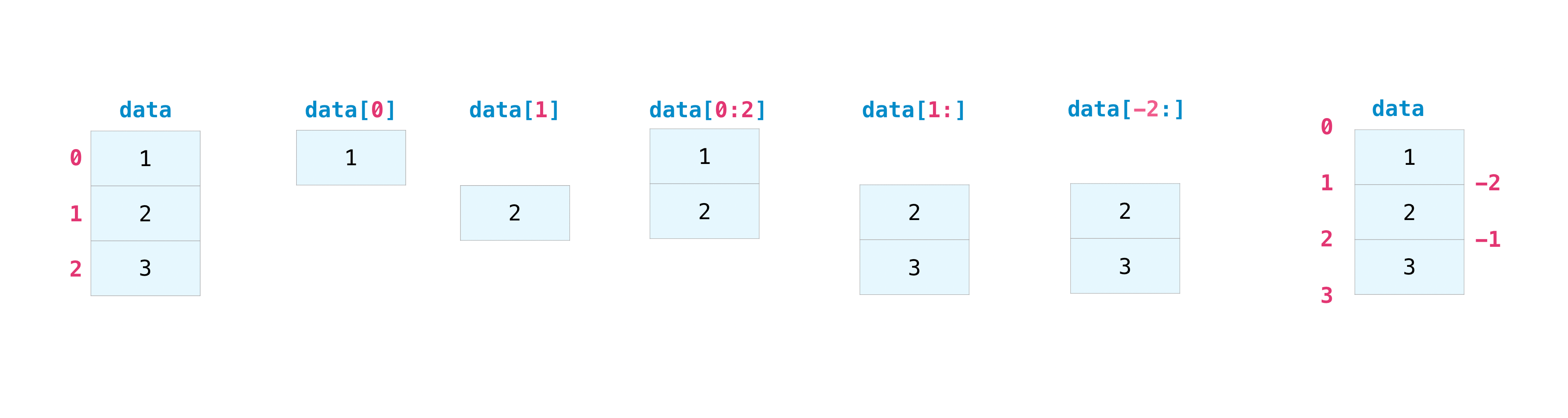
You may want to take a section of your array or specific assortment elements to utilize in further analysis or boosted operations. To practise that, yous'll demand to subset, piece, and/or index your arrays.
If you want to select values from your array that fulfill certain conditions, it's straightforward with NumPy.
For example, if you start with this assortment:
>>> a = np . array ([[ 1 , 2 , iii , 4 ], [ v , 6 , 7 , eight ], [ ix , 10 , 11 , 12 ]]) You can easily print all of the values in the array that are less than v.
>>> print ( a [ a < v ]) [i 2 3 4] You tin can likewise select, for example, numbers that are equal to or greater than 5, and use that condition to alphabetize an array.
>>> five_up = ( a >= 5 ) >>> print ( a [ five_up ]) [ 5 6 7 eight 9 10 xi 12] Yous can select elements that are divisible past two:
>>> divisible_by_2 = a [ a % 2 == 0 ] >>> print ( divisible_by_2 ) [ 2 iv 6 viii 10 12] Or yous can select elements that satisfy two conditions using the & and | operators:
>>> c = a [( a > 2 ) & ( a < 11 )] >>> print ( c ) [ iii 4 five half dozen 7 eight 9 ten] You can also make use of the logical operators & and | in order to render boolean values that specify whether or not the values in an array fulfill a certain status. This can be useful with arrays that contain names or other chiselled values.
>>> five_up = ( a > 5 ) | ( a == 5 ) >>> impress ( five_up ) [[Imitation False False False] [ Truthful True True Truthful] [ Truthful Truthful True Truthful]] You can also use np.nonzero() to select elements or indices from an array.
Starting with this array:
>>> a = np . array ([[ 1 , 2 , 3 , iv ], [ 5 , 6 , vii , 8 ], [ 9 , ten , 11 , 12 ]]) You can use np.nonzero() to print the indices of elements that are, for case, less than 5:
>>> b = np . nonzero ( a < 5 ) >>> print ( b ) (assortment([0, 0, 0, 0]), array([0, 1, ii, three])) In this case, a tuple of arrays was returned: one for each dimension. The first array represents the row indices where these values are found, and the second array represents the column indices where the values are plant.
If y'all want to generate a list of coordinates where the elements exist, y'all can zip the arrays, iterate over the listing of coordinates, and print them. For instance:
>>> list_of_coordinates = list ( cypher ( b [ 0 ], b [ 1 ])) >>> for coord in list_of_coordinates : ... print ( coord ) (0, 0) (0, 1) (0, 2) (0, iii) Yous tin as well employ np.nonzero() to print the elements in an array that are less than 5 with:
>>> print ( a [ b ]) [ane 2 3 4] If the element yous're looking for doesn't exist in the assortment, and then the returned array of indices will be empty. For example:
>>> not_there = np . nonzero ( a == 42 ) >>> print ( not_there ) (assortment([], dtype=int64), array([], dtype=int64)) Acquire more about indexing and slicing here and here.
Read more about using the nonzero part at: nonzero .
How to create an array from existing data
This department covers slicing and indexing , np.vstack() , np.hstack() , np.hsplit() , .view() , copy()
Y'all can hands create a new assortment from a section of an existing assortment.
Allow's say you lot take this assortment:
>>> a = np . array ([ 1 , 2 , 3 , 4 , five , 6 , 7 , eight , 9 , 10 ]) Y'all can create a new array from a section of your array any time by specifying where yous want to piece your array.
>>> arr1 = a [ three : 8 ] >>> arr1 array([4, 5, 6, 7, 8]) Here, you grabbed a section of your array from index position three through index position 8.
You can also stack 2 existing arrays, both vertically and horizontally. Let's say y'all have two arrays, a1 and a2 :
>>> a1 = np . array ([[ ane , one ], ... [ 2 , ii ]]) >>> a2 = np . array ([[ 3 , 3 ], ... [ 4 , four ]]) You can stack them vertically with vstack :
>>> np . vstack (( a1 , a2 )) array([[i, 1], [2, 2], [three, 3], [4, 4]]) Or stack them horizontally with hstack :
>>> np . hstack (( a1 , a2 )) array([[ane, one, three, 3], [2, two, 4, four]]) You can split an array into several smaller arrays using hsplit . You can specify either the number of equally shaped arrays to return or the columns after which the division should occur.
Let's say you lot have this array:
>>> x = np . arange ( 1 , 25 ) . reshape ( two , 12 ) >>> x array([[ 1, 2, 3, iv, five, 6, 7, 8, nine, 10, 11, 12], [thirteen, 14, xv, 16, 17, 18, nineteen, twenty, 21, 22, 23, 24]]) If yous wanted to separate this array into 3 equally shaped arrays, you would run:
>>> np . hsplit ( x , 3 ) [array([[ 1, two, three, 4], [13, fourteen, fifteen, 16]]), assortment([[ v, six, 7, eight], [17, 18, 19, 20]]), array([[ nine, 10, 11, 12], [21, 22, 23, 24]])] If you lot wanted to dissever your array after the tertiary and fourth column, yous'd run:
>>> np . hsplit ( x , ( 3 , 4 )) [assortment([[ 1, 2, iii], [thirteen, fourteen, xv]]), array([[ iv], [16]]), array([[ 5, vi, 7, 8, 9, x, 11, 12], [17, xviii, 19, 20, 21, 22, 23, 24]])] Larn more than about stacking and splitting arrays hither.
You can utilize the view method to create a new assortment object that looks at the same information equally the original array (a shallow re-create).
Views are an important NumPy concept! NumPy functions, besides as operations like indexing and slicing, will return views whenever possible. This saves retentivity and is faster (no copy of the data has to be fabricated). However information technology'due south important to be aware of this - modifying data in a view as well modifies the original array!
Permit's say you create this array:
>>> a = np . array ([[ 1 , 2 , iii , four ], [ 5 , 6 , 7 , 8 ], [ 9 , 10 , 11 , 12 ]]) At present nosotros create an array b1 by slicing a and modify the first element of b1 . This volition modify the corresponding element in a also!
>>> b1 = a [ 0 , :] >>> b1 array([ane, ii, 3, 4]) >>> b1 [ 0 ] = 99 >>> b1 assortment([99, 2, 3, iv]) >>> a array([[99, ii, 3, 4], [ 5, 6, 7, viii], [ 9, 10, 11, 12]]) Using the re-create method will make a consummate re-create of the assortment and its data (a deep copy). To utilise this on your array, you could run:
Learn more about copies and views here.
Bones array operations
This section covers improver, subtraction, multiplication, division, and more
In one case y'all've created your arrays, you lot can start to work with them. Let's say, for example, that y'all've created 2 arrays, one called "data" and one called "ones"
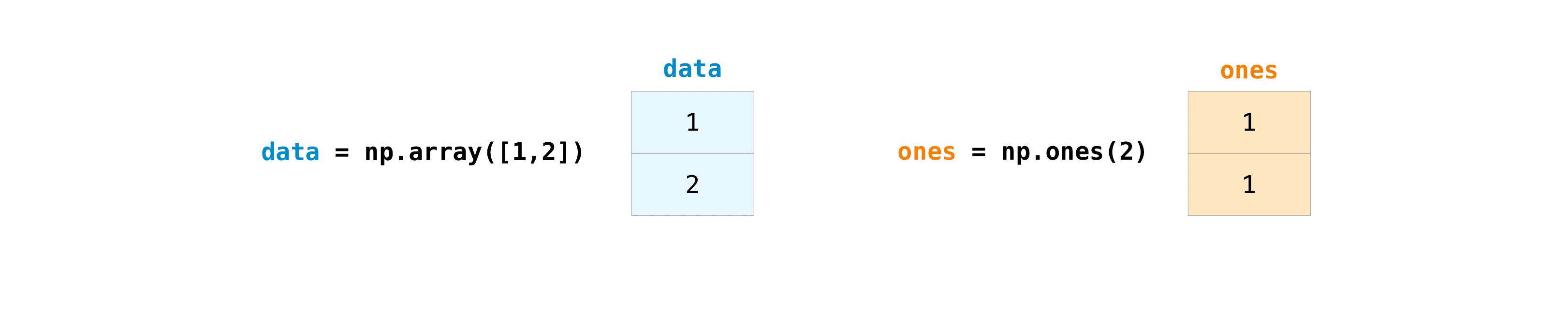
You can add the arrays together with the plus sign.
>>> data = np . array ([ 1 , 2 ]) >>> ones = np . ones ( 2 , dtype = int ) >>> information + ones assortment([two, 3]) 
You can, of grade, do more than just addition!
>>> data - ones array([0, i]) >>> information * data assortment([i, 4]) >>> data / information array([1., 1.]) 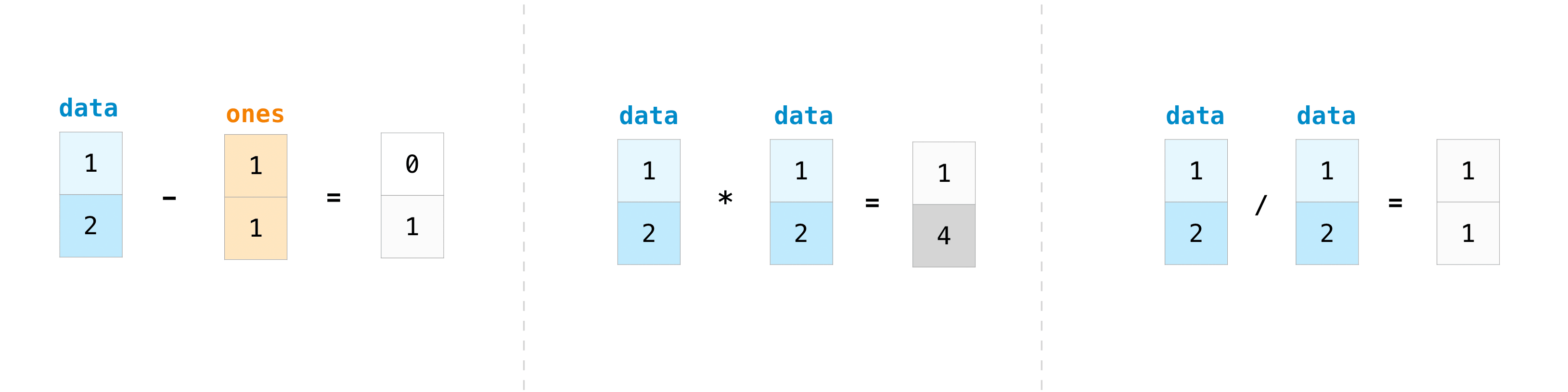
Basic operations are simple with NumPy. If you want to find the sum of the elements in an assortment, y'all'd use sum() . This works for 1D arrays, 2d arrays, and arrays in college dimensions.
>>> a = np . array ([ 1 , 2 , three , 4 ]) >>> a . sum () 10 To add the rows or the columns in a 2D assortment, you would specify the axis.
If you showtime with this array:
>>> b = np . array ([[ one , ane ], [ 2 , 2 ]]) You lot can sum over the axis of rows with:
>>> b . sum ( axis = 0 ) array([3, 3]) You tin sum over the axis of columns with:
>>> b . sum ( axis = one ) assortment([ii, 4]) Learn more than about bones operations hither.
Broadcasting
In that location are times when you might want to carry out an operation between an array and a single number (also called an performance between a vector and a scalar) or between arrays of two dissimilar sizes. For example, your assortment (we'll call it "data") might incorporate information about altitude in miles just you want to convert the information to kilometers. You tin can perform this operation with:
>>> data = np . array ([ i.0 , 2.0 ]) >>> data * 1.6 array([1.6, 3.2]) 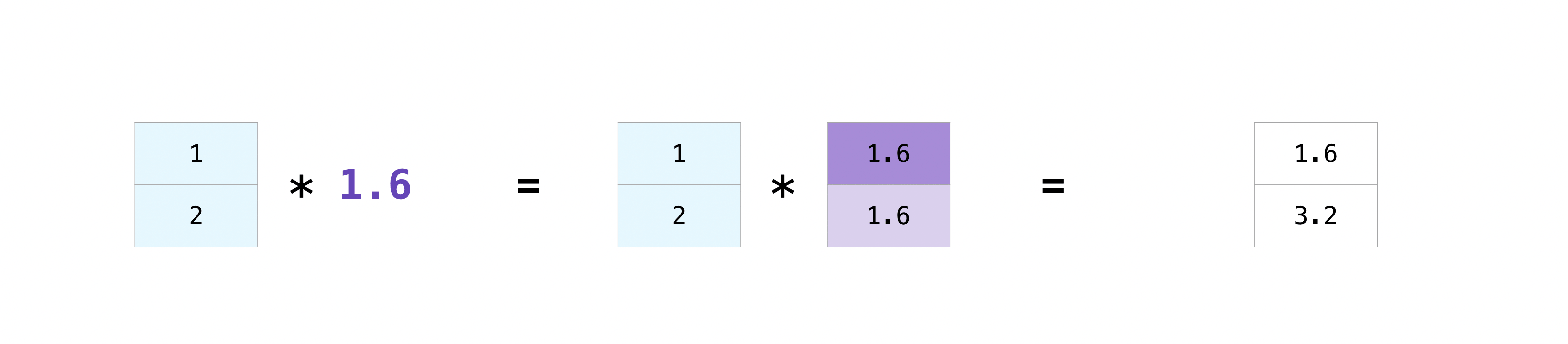
NumPy understands that the multiplication should happen with each cell. That concept is called broadcasting. Broadcasting is a mechanism that allows NumPy to perform operations on arrays of different shapes. The dimensions of your array must be compatible, for example, when the dimensions of both arrays are equal or when 1 of them is 1. If the dimensions are not uniform, you lot will get a ValueError .
Larn more than about broadcasting here.
More useful array operations
This section covers maximum, minimum, sum, mean, product, standard deviation, and more than
NumPy also performs aggregation functions. In addition to min , max , and sum , you tin can easily run mean to get the average, prod to get the outcome of multiplying the elements together, std to get the standard deviation, and more.
>>> data . max () ii.0 >>> data . min () 1.0 >>> data . sum () 3.0 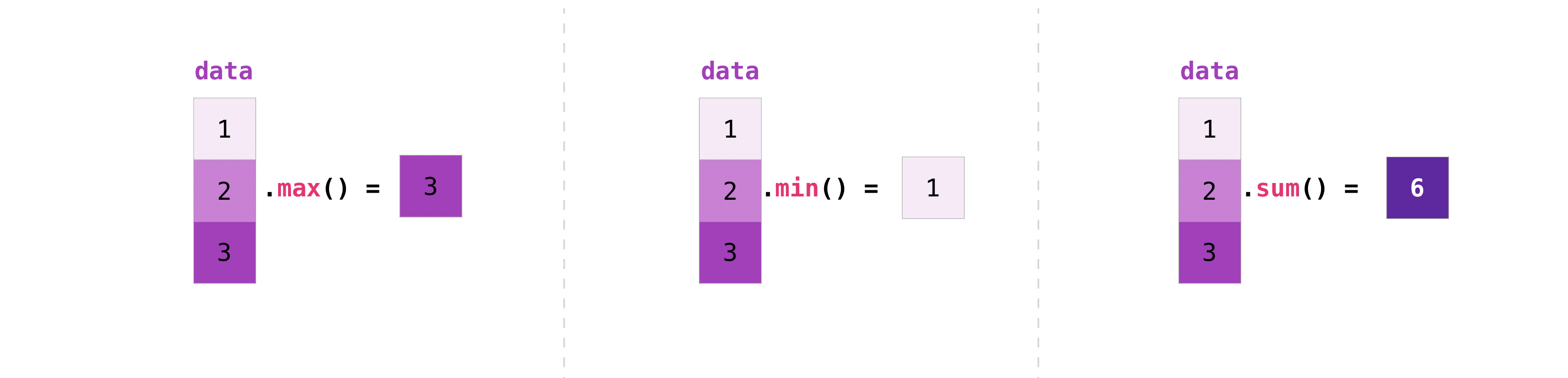
Allow's start with this assortment, called "a"
>>> a = np . array ([[ 0.45053314 , 0.17296777 , 0.34376245 , 0.5510652 ], ... [ 0.54627315 , 0.05093587 , 0.40067661 , 0.55645993 ], ... [ 0.12697628 , 0.82485143 , 0.26590556 , 0.56917101 ]]) It'southward very common to want to amass along a row or cavalcade. By default, every NumPy assemblage role volition return the amass of the entire array. To find the sum or the minimum of the elements in your array, run:
Or:
You can specify on which axis you want the aggregation part to be computed. For example, you tin find the minimum value within each column by specifying axis=0 .
>>> a . min ( axis = 0 ) assortment([0.12697628, 0.05093587, 0.26590556, 0.5510652 ]) The 4 values listed higher up represent to the number of columns in your array. With a four-column array, you will get 4 values equally your effect.
Read more than about assortment methods hither.
Creating matrices
Y'all can laissez passer Python lists of lists to create a 2-D array (or "matrix") to represent them in NumPy.
>>> data = np . array ([[ one , 2 ], [ 3 , 4 ], [ 5 , half-dozen ]]) >>> data array([[1, 2], [iii, four], [5, 6]]) 
Indexing and slicing operations are useful when you're manipulating matrices:
>>> data [ 0 , ane ] 2 >>> data [ 1 : 3 ] assortment([[3, 4], [five, six]]) >>> information [ 0 : ii , 0 ] assortment([1, 3]) 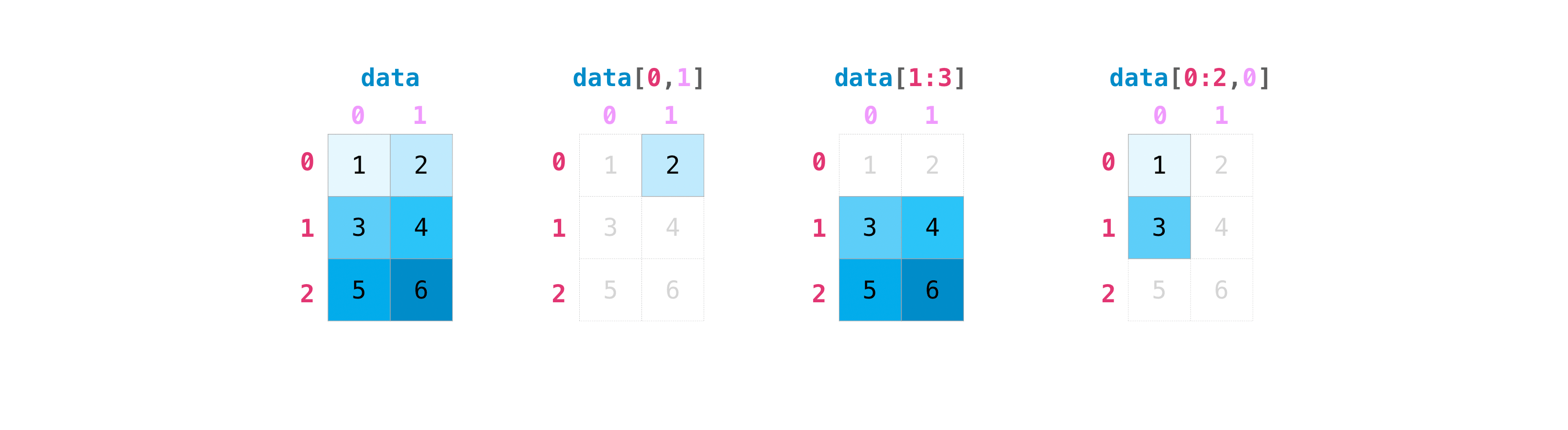
You tin amass matrices the same manner you aggregated vectors:
>>> data . max () 6 >>> information . min () 1 >>> data . sum () 21 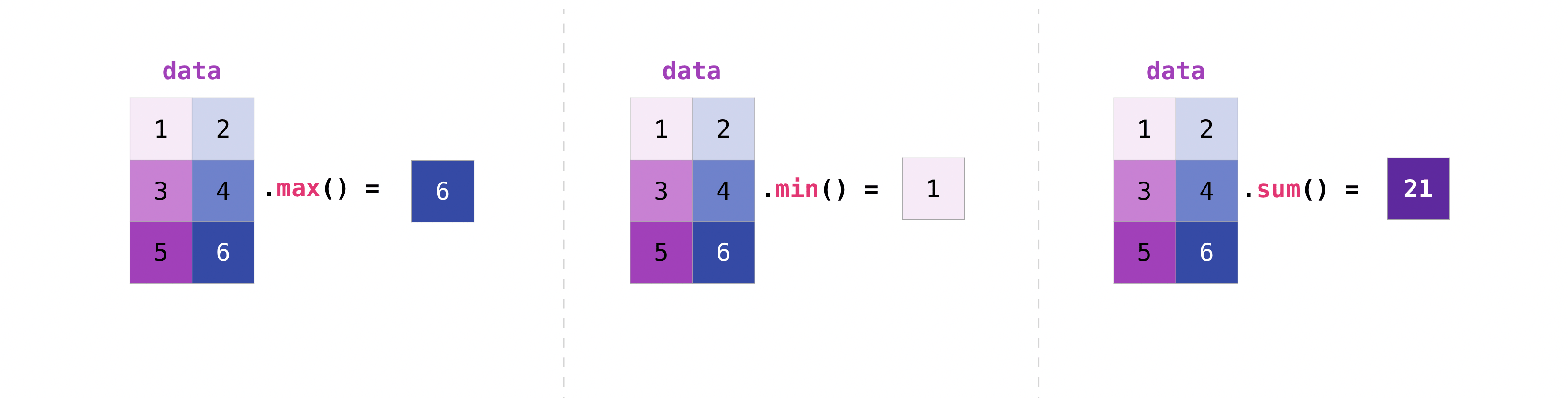
Yous can aggregate all the values in a matrix and you can amass them beyond columns or rows using the centrality parameter. To illustrate this bespeak, permit'southward look at a slightly modified dataset:
>>> data = np . array ([[ 1 , 2 ], [ 5 , 3 ], [ 4 , 6 ]]) >>> data assortment([[1, 2], [v, iii], [4, 6]]) >>> data . max ( axis = 0 ) array([5, half-dozen]) >>> data . max ( centrality = 1 ) array([2, 5, half-dozen]) 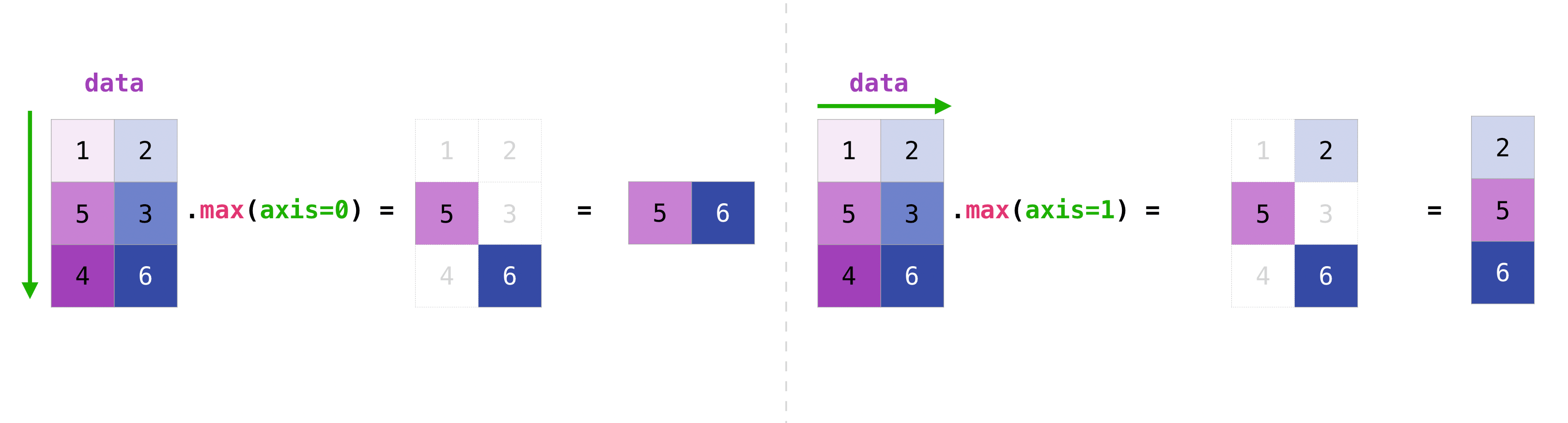
One time you've created your matrices, you can add and multiply them using arithmetic operators if you lot accept two matrices that are the same size.
>>> data = np . array ([[ 1 , 2 ], [ 3 , 4 ]]) >>> ones = np . array ([[ 1 , ane ], [ 1 , one ]]) >>> data + ones array([[two, 3], [4, v]]) 
You lot can practise these arithmetic operations on matrices of different sizes, but only if one matrix has only ane column or ane row. In this case, NumPy will use its broadcast rules for the functioning.
>>> data = np . assortment ([[ one , two ], [ 3 , 4 ], [ 5 , 6 ]]) >>> ones_row = np . assortment ([[ i , 1 ]]) >>> data + ones_row array([[ii, 3], [4, 5], [6, 7]]) 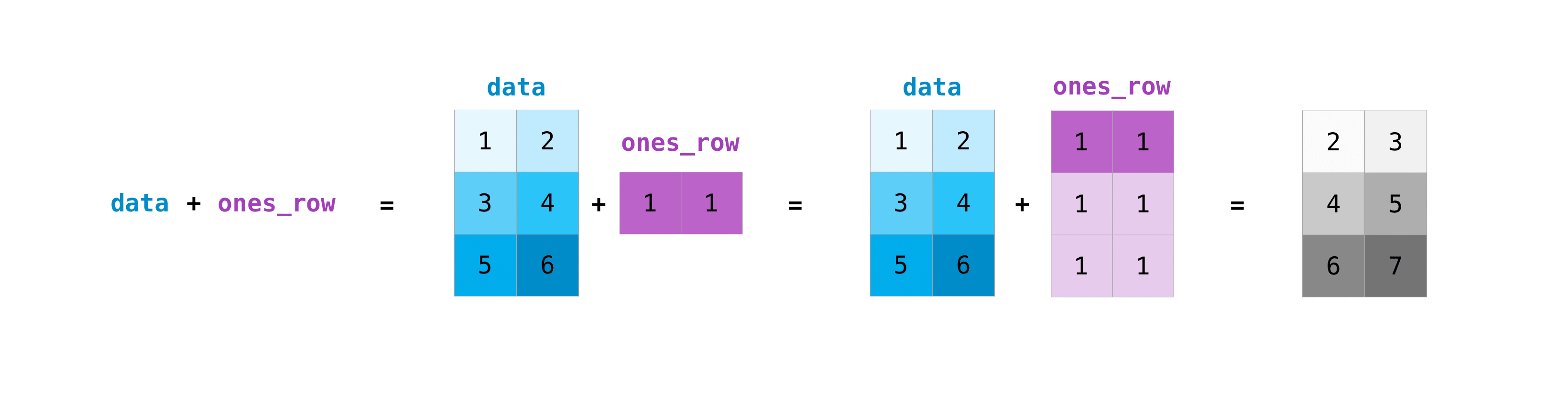
Exist aware that when NumPy prints Due north-dimensional arrays, the last axis is looped over the fastest while the offset axis is the slowest. For instance:
>>> np . ones (( 4 , 3 , ii )) assortment([[[ane., 1.], [1., 1.], [1., 1.]], [[1., one.], [i., 1.], [1., 1.]], [[1., 1.], [1., 1.], [one., 1.]], [[ane., one.], [1., ane.], [1., 1.]]]) There are often instances where nosotros want NumPy to initialize the values of an array. NumPy offers functions similar ones() and zeros() , and the random.Generator class for random number generation for that. All you lot demand to exercise is pass in the number of elements you lot desire it to generate:
>>> np . ones ( 3 ) array([1., one., 1.]) >>> np . zeros ( iii ) assortment([0., 0., 0.]) >>> rng = np . random . default_rng () # the simplest way to generate random numbers >>> rng . random ( 3 ) array([0.63696169, 0.26978671, 0.04097352]) 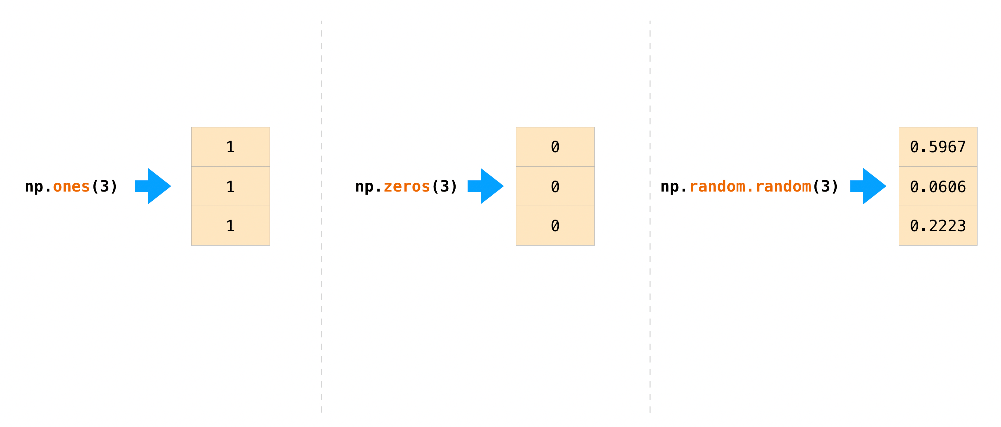
You can also use ones() , zeros() , and random() to create a 2D array if you requite them a tuple describing the dimensions of the matrix:
>>> np . ones (( 3 , two )) array([[1., 1.], [1., 1.], [1., 1.]]) >>> np . zeros (( three , 2 )) array([[0., 0.], [0., 0.], [0., 0.]]) >>> rng . random (( 3 , 2 )) assortment([[0.01652764, 0.81327024], [0.91275558, 0.60663578], [0.72949656, 0.54362499]]) # may vary 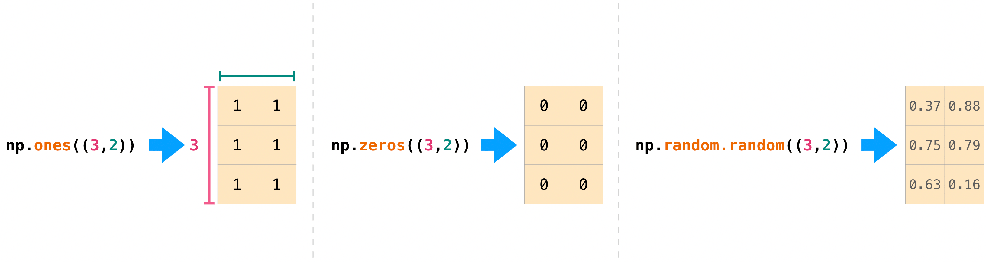
Read more well-nigh creating arrays, filled with 0 's, 1 's, other values or uninitialized, at array cosmos routines.
Generating random numbers
The utilise of random number generation is an important part of the configuration and evaluation of many numerical and auto learning algorithms. Whether you demand to randomly initialize weights in an artificial neural network, split data into random sets, or randomly shuffle your dataset, existence able to generate random numbers (actually, repeatable pseudo-random numbers) is essential.
With Generator.integers , yous tin generate random integers from low (call up that this is inclusive with NumPy) to high (exclusive). You tin ready endpoint=True to make the high number inclusive.
You tin generate a two x iv array of random integers betwixt 0 and 4 with:
>>> rng . integers ( 5 , size = ( ii , 4 )) array([[ii, 1, ane, 0], [0, 0, 0, four]]) # may vary Read more about random number generation here.
How to go unique items and counts
This section covers np.unique()
You can notice the unique elements in an assortment easily with np.unique .
For example, if you offset with this array:
>>> a = np . assortment ([ 11 , 11 , 12 , 13 , 14 , xv , 16 , 17 , 12 , xiii , 11 , 14 , 18 , 19 , 20 ]) y'all tin can use np.unique to print the unique values in your assortment:
>>> unique_values = np . unique ( a ) >>> print ( unique_values ) [11 12 13 14 15 16 17 18 19 xx] To get the indices of unique values in a NumPy array (an array of beginning index positions of unique values in the array), just pass the return_index argument in np.unique() as well as your array.
>>> unique_values , indices_list = np . unique ( a , return_index = True ) >>> print ( indices_list ) [ 0 2 iii 4 5 6 vii 12 13 14] Y'all tin pass the return_counts argument in np.unique() forth with your assortment to get the frequency count of unique values in a NumPy array.
>>> unique_values , occurrence_count = np . unique ( a , return_counts = True ) >>> print ( occurrence_count ) [three 2 2 2 1 ane i 1 1 1] This also works with 2D arrays! If y'all start with this array:
>>> a_2d = np . assortment ([[ i , ii , 3 , iv ], [ v , six , 7 , viii ], [ 9 , 10 , 11 , 12 ], [ one , 2 , iii , 4 ]]) You tin detect unique values with:
>>> unique_values = np . unique ( a_2d ) >>> impress ( unique_values ) [ one ii 3 iv five 6 vii 8 9 10 11 12] If the axis argument isn't passed, your 2D array will be flattened.
If you want to become the unique rows or columns, make certain to laissez passer the axis argument. To find the unique rows, specify centrality=0 and for columns, specify axis=i .
>>> unique_rows = np . unique ( a_2d , axis = 0 ) >>> print ( unique_rows ) [[ i 2 three 4] [ 5 six 7 8] [ 9 x xi 12]] To go the unique rows, index position, and occurrence count, you tin can use:
>>> unique_rows , indices , occurrence_count = np . unique ( ... a_2d , centrality = 0 , return_counts = True , return_index = True ) >>> print ( unique_rows ) [[ 1 two three 4] [ 5 half-dozen 7 8] [ 9 10 11 12]] >>> print ( indices ) [0 one 2] >>> print ( occurrence_count ) [2 i i] To learn more about finding the unique elements in an array, encounter unique .
Transposing and reshaping a matrix
This section covers arr.reshape() , arr.transpose() , arr.T
It'due south common to need to transpose your matrices. NumPy arrays have the property T that allows you to transpose a matrix.

You may besides need to switch the dimensions of a matrix. This can happen when, for case, y'all have a model that expects a certain input shape that is different from your dataset. This is where the reshape method tin can exist useful. You simply need to pass in the new dimensions that you want for the matrix.
>>> data . reshape ( 2 , three ) array([[one, 2, iii], [4, v, vi]]) >>> data . reshape ( three , 2 ) assortment([[1, 2], [iii, four], [5, 6]]) 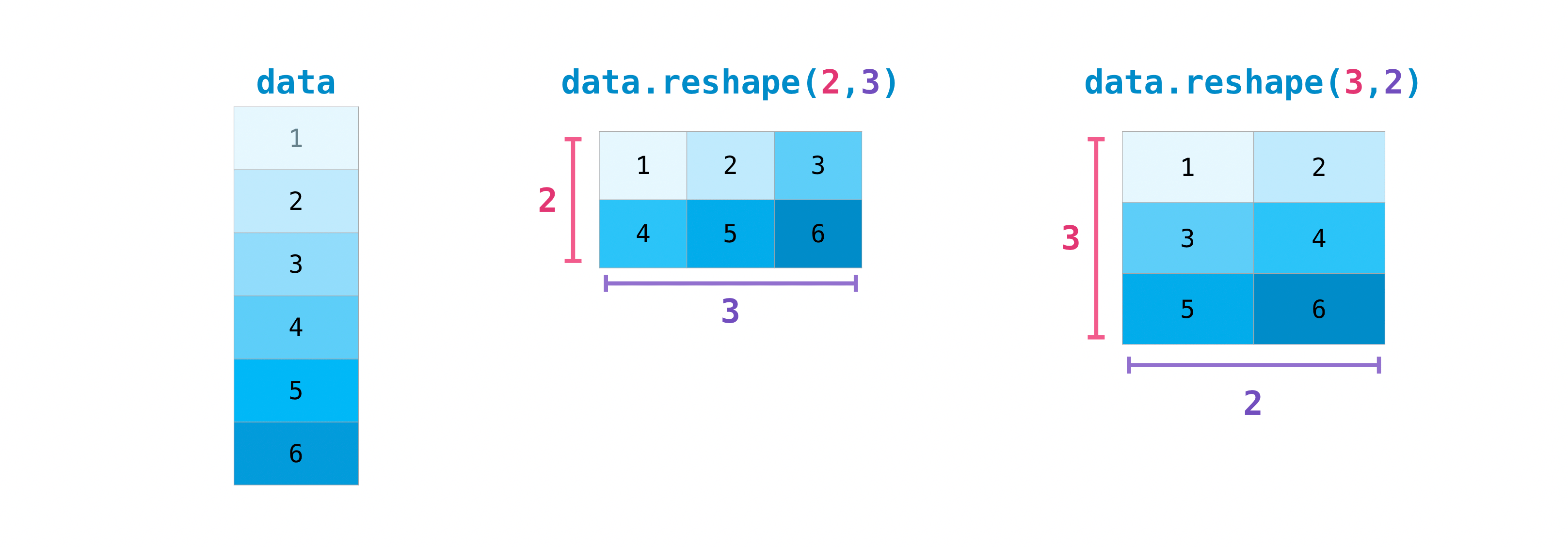
You can also use .transpose() to reverse or change the axes of an assortment according to the values you lot specify.
If you start with this array:
>>> arr = np . arange ( 6 ) . reshape (( 2 , 3 )) >>> arr array([[0, 1, 2], [3, iv, v]]) You tin transpose your array with arr.transpose() .
>>> arr . transpose () array([[0, iii], [i, 4], [2, 5]]) Yous can also use arr.T :
>>> arr . T array([[0, 3], [1, iv], [2, five]]) To learn more well-nigh transposing and reshaping arrays, see transpose and reshape .
How to reverse an array
This section covers np.flip()
NumPy'southward np.flip() office allows you lot to flip, or reverse, the contents of an array along an axis. When using np.flip() , specify the assortment you would like to contrary and the axis. If you don't specify the axis, NumPy volition reverse the contents along all of the axes of your input array.
Reversing a 1D assortment
If y'all begin with a 1D array like this 1:
>>> arr = np . array ([ ane , 2 , iii , 4 , 5 , 6 , seven , 8 ]) You lot tin can reverse it with:
>>> reversed_arr = np . flip ( arr ) If you want to impress your reversed array, y'all tin run:
>>> print ( 'Reversed Assortment: ' , reversed_arr ) Reversed Array: [viii 7 6 5 iv 3 2 i] Reversing a 2D array
A second array works much the same way.
If yous start with this assortment:
>>> arr_2d = np . array ([[ 1 , two , 3 , 4 ], [ 5 , 6 , 7 , 8 ], [ nine , 10 , 11 , 12 ]]) Y'all tin can reverse the content in all of the rows and all of the columns with:
>>> reversed_arr = np . flip ( arr_2d ) >>> print ( reversed_arr ) [[12 11 10 9] [ 8 seven six 5] [ 4 3 ii 1]] You can easily reverse only the rows with:
>>> reversed_arr_rows = np . flip ( arr_2d , axis = 0 ) >>> print ( reversed_arr_rows ) [[ 9 x 11 12] [ 5 6 7 8] [ 1 2 iii 4]] Or reverse simply the columns with:
>>> reversed_arr_columns = np . flip ( arr_2d , axis = 1 ) >>> print ( reversed_arr_columns ) [[ 4 3 two 1] [ 8 7 6 5] [12 eleven x 9]] You can also reverse the contents of merely i cavalcade or row. For example, you tin can opposite the contents of the row at alphabetize position 1 (the 2d row):
>>> arr_2d [ 1 ] = np . flip ( arr_2d [ 1 ]) >>> impress ( arr_2d ) [[ ane 2 3 4] [ 8 7 6 5] [ 9 10 11 12]] You tin can also reverse the cavalcade at alphabetize position 1 (the 2d column):
>>> arr_2d [:, 1 ] = np . flip ( arr_2d [:, i ]) >>> print ( arr_2d ) [[ 1 10 3 four] [ eight 7 6 5] [ 9 2 11 12]] Read more most reversing arrays at flip .
Reshaping and flattening multidimensional arrays
This section covers .flatten() , ravel()
There are ii popular ways to flatten an array: .flatten() and .ravel() . The principal difference between the 2 is that the new array created using ravel() is really a reference to the parent array (i.e., a "view"). This means that any changes to the new array will affect the parent array too. Since ravel does non create a copy, it's memory efficient.
If you start with this array:
>>> x = np . array ([[ 1 , ii , 3 , iv ], [ 5 , six , 7 , viii ], [ nine , 10 , xi , 12 ]]) You can use flatten to flatten your assortment into a 1D array.
>>> ten . flatten () array([ 1, ii, 3, 4, 5, half dozen, 7, 8, ix, 10, 11, 12]) When you employ flatten , changes to your new array won't change the parent assortment.
For case:
>>> a1 = x . flatten () >>> a1 [ 0 ] = 99 >>> print ( ten ) # Original array [[ 1 two 3 four] [ five six 7 eight] [ nine 10 xi 12]] >>> print ( a1 ) # New array [99 2 3 four five 6 7 8 9 ten 11 12] But when you use ravel , the changes you make to the new assortment will affect the parent array.
For example:
>>> a2 = x . ravel () >>> a2 [ 0 ] = 98 >>> impress ( x ) # Original array [[98 2 3 4] [ 5 six 7 8] [ 9 10 11 12]] >>> print ( a2 ) # New assortment [98 2 iii iv 5 6 7 8 9 10 eleven 12] Read more about flatten at ndarray.flatten and ravel at ravel .
How to access the docstring for more information
This section covers help() , ? , ??
When information technology comes to the data science ecosystem, Python and NumPy are built with the user in listen. One of the best examples of this is the congenital-in access to documentation. Every object contains the reference to a string, which is known as the docstring. In most cases, this docstring contains a quick and concise summary of the object and how to utilise information technology. Python has a built-in help() office that can assist you access this information. This means that well-nigh whatsoever time yous need more information, you can employ help() to quickly find the information that you lot need.
For case:
>>> help ( max ) Help on congenital-in function max in module builtins: max(...) max(iterable, *[, default=obj, key=func]) -> value max(arg1, arg2, *args, *[, key=func]) -> value With a single iterable argument, return its biggest item. The default keyword-only argument specifies an object to return if the provided iterable is empty. With ii or more arguments, render the largest argument. Because admission to additional information is so useful, IPython uses the ? character as a autograph for accessing this documentation forth with other relevant data. IPython is a command shell for interactive calculating in multiple languages. Y'all can find more information nigh IPython here.
For example:
In [0]: max? max(iterable, *[, default=obj, key=func]) -> value max(arg1, arg2, *args, *[, key=func]) -> value With a single iterable argument, return its biggest detail. The default keyword-only argument specifies an object to return if the provided iterable is empty. With two or more arguments, return the largest argument. Type: builtin_function_or_method You can even use this notation for object methods and objects themselves.
Let's say you create this array:
>>> a = np . array ([ ane , 2 , three , 4 , 5 , half-dozen ]) And so you can obtain a lot of useful data (first details about a itself, followed by the docstring of ndarray of which a is an example):
In [i]: a? Type: ndarray String form: [i two 3 4 five six] Length: six File: ~/anaconda3/lib/python3.7/site-packages/numpy/__init__.py Docstring: <no docstring> Course docstring: ndarray(shape, dtype=float, buffer=None, get-go=0, strides=None, order=None) An array object represents a multidimensional, homogeneous assortment of fixed-size items. An associated data-type object describes the format of each element in the array (its byte-club, how many bytes information technology occupies in retentivity, whether it is an integer, a floating point number, or something else, etc.) Arrays should be synthetic using `assortment`, `zeros` or `empty` (refer to the See Likewise section below). The parameters given here refer to a low-level method (`ndarray(...)`) for instantiating an array. For more information, refer to the `numpy` module and examine the methods and attributes of an array. Parameters ---------- ( for the __new__ method ; run across Notes beneath ) shape : tuple of ints Shape of created array . ... This besides works for functions and other objects that you create. Just remember to include a docstring with your function using a cord literal ( """ """ or ''' ''' effectually your documentation).
For example, if you create this function:
>>> def double ( a ): ... '''Return a * ii''' ... render a * ii You can obtain information almost the role:
In [two]: double? Signature: double(a) Docstring: Render a * 2 File: ~/Desktop/<ipython-input-23-b5adf20be596> Type: function You lot can accomplish another level of information by reading the source code of the object you're interested in. Using a double question mark ( ?? ) allows y'all to access the source code.
For example:
In [3]: double?? Signature: double(a) Source: def double(a): '''Return a * 2''' return a * two File: ~/Desktop/<ipython-input-23-b5adf20be596> Type: part If the object in question is compiled in a language other than Python, using ?? will return the same information as ? . You'll observe this with a lot of congenital-in objects and types, for example:
In [4]: len? Signature: len(obj, /) Docstring: Return the number of items in a container. Blazon: builtin_function_or_method and :
In [5]: len?? Signature: len(obj, /) Docstring: Return the number of items in a container. Type: builtin_function_or_method have the aforementioned output because they were compiled in a programming language other than Python.
Working with mathematical formulas
The ease of implementing mathematical formulas that piece of work on arrays is 1 of the things that make NumPy and so widely used in the scientific Python customs.
For instance, this is the mean square error formula (a fundamental formula used in supervised machine learning models that bargain with regression):
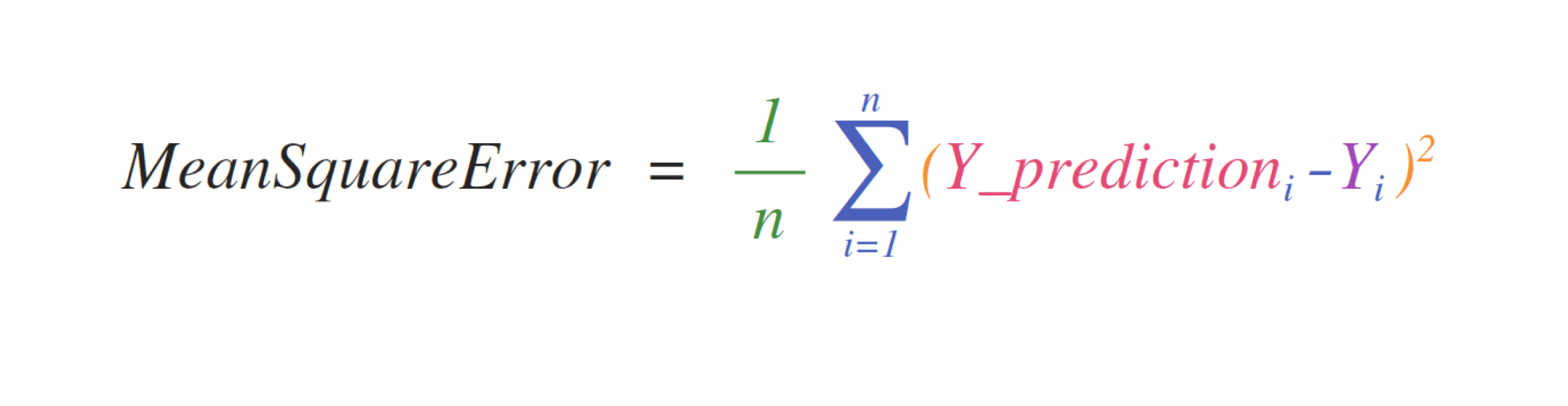
Implementing this formula is unproblematic and straightforward in NumPy:
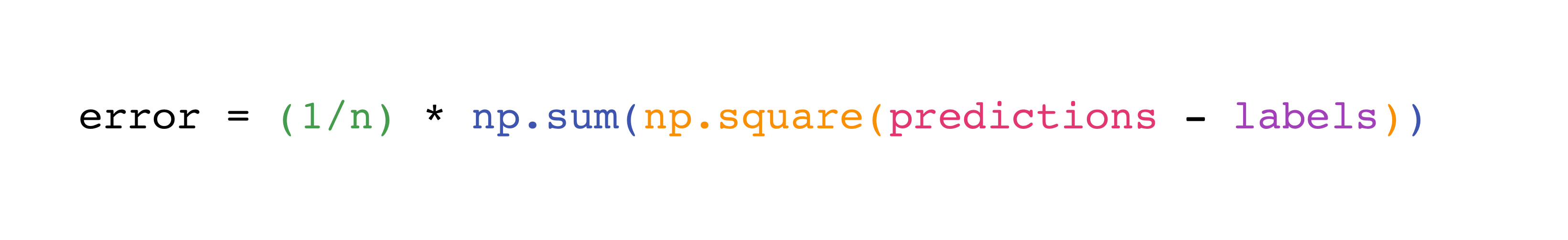
What makes this work so well is that predictions and labels can incorporate one or a grand values. They merely need to be the same size.
Y'all can visualize it this way:
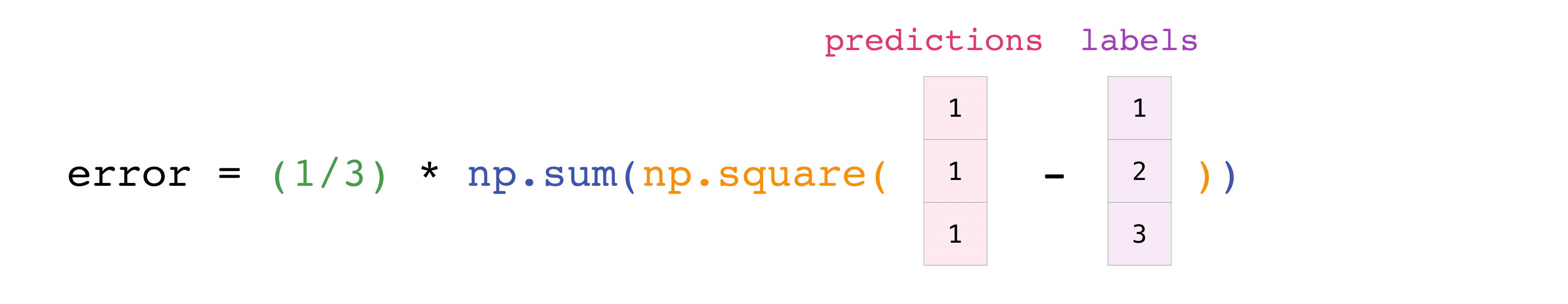
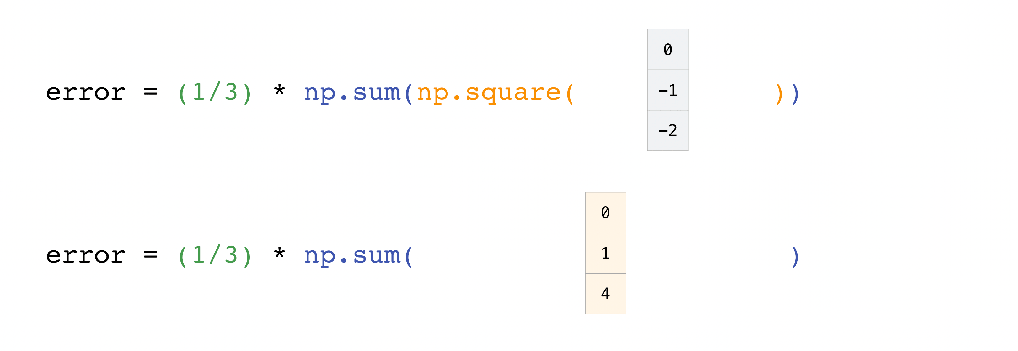
In this instance, both the predictions and labels vectors contain three values, meaning n has a value of iii. After we carry out subtractions the values in the vector are squared. And so NumPy sums the values, and your issue is the fault value for that prediction and a score for the quality of the model.

How to salve and load NumPy objects
This section covers np.save , np.savez , np.savetxt , np.load , np.loadtxt
Y'all volition, at some point, want to salvage your arrays to deejay and load them dorsum without having to re-run the code. Fortunately, there are several ways to save and load objects with NumPy. The ndarray objects tin can exist saved to and loaded from the disk files with loadtxt and savetxt functions that handle normal text files, load and salve functions that handle NumPy binary files with a .npy file extension, and a savez function that handles NumPy files with a .npz file extension.
The .npy and .npz files store data, shape, dtype, and other information required to reconstruct the ndarray in a style that allows the array to be correctly retrieved, even when the file is on some other machine with unlike architecture.
If you lot want to shop a single ndarray object, store information technology as a .npy file using np.save . If y'all want to store more than one ndarray object in a single file, save it as a .npz file using np.savez . You tin as well relieve several arrays into a unmarried file in compressed npz format with savez_compressed .
It'south easy to save and load and array with np.relieve() . Only make sure to specify the array you want to save and a file name. For example, if you create this assortment:
>>> a = np . array ([ one , 2 , iii , 4 , 5 , 6 ]) You tin save it as "filename.npy" with:
>>> np . save ( 'filename' , a ) Yous tin use np.load() to reconstruct your array.
>>> b = np . load ( 'filename.npy' ) If you want to check your array, you tin run::
>>> print ( b ) [1 2 3 4 v vi] You can salvage a NumPy array as a plain text file like a .csv or .txt file with np.savetxt .
For example, if you create this array:
>>> csv_arr = np . array ([ 1 , two , three , iv , five , 6 , 7 , 8 ]) Y'all tin hands salvage information technology every bit a .csv file with the proper noun "new_file.csv" like this:
>>> np . savetxt ( 'new_file.csv' , csv_arr ) You tin can chop-chop and easily load your saved text file using loadtxt() :
>>> np . loadtxt ( 'new_file.csv' ) assortment([1., 2., iii., 4., 5., 6., 7., 8.]) The savetxt() and loadtxt() functions take boosted optional parameters such every bit header, footer, and delimiter. While text files tin can be easier for sharing, .npy and .npz files are smaller and faster to read. If y'all need more sophisticated treatment of your text file (for instance, if you lot need to work with lines that contain missing values), y'all will want to use the genfromtxt part.
With savetxt , you can specify headers, footers, comments, and more than.
Learn more virtually input and output routines here.
Importing and exporting a CSV
It's simple to read in a CSV that contains existing data. The best and easiest way to exercise this is to utilize Pandas.
>>> import pandas as pd >>> # If all of your columns are the same blazon: >>> x = pd . read_csv ( 'music.csv' , header = 0 ) . values >>> print ( 10 ) [['Billie Holiday' 'Jazz' 1300000 27000000] ['Jimmie Hendrix' 'Stone' 2700000 70000000] ['Miles Davis' 'Jazz' 1500000 48000000] ['SIA' 'Pop' 2000000 74000000]] >>> # You lot tin also but select the columns you lot need: >>> x = pd . read_csv ( 'music.csv' , usecols = [ 'Artist' , 'Plays' ]) . values >>> print ( x ) [['Billie Holiday' 27000000] ['Jimmie Hendrix' 70000000] ['Miles Davis' 48000000] ['SIA' 74000000]] 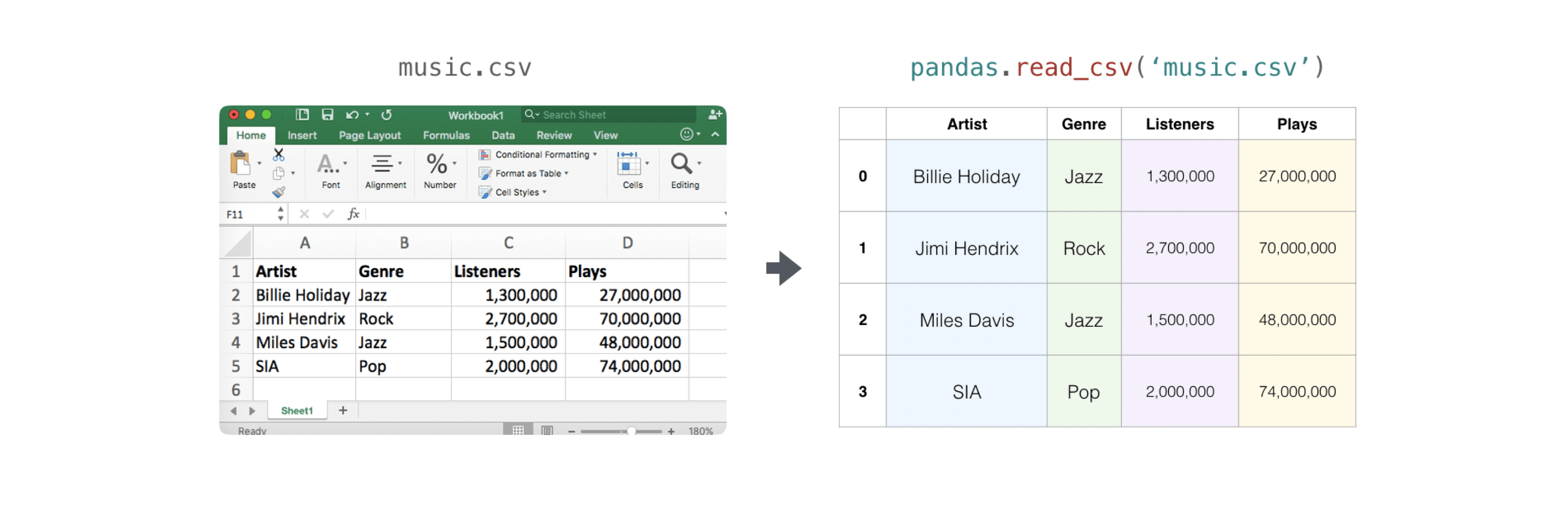
It's simple to use Pandas in society to export your assortment as well. If you are new to NumPy, you may desire to create a Pandas dataframe from the values in your array and so write the data frame to a CSV file with Pandas.
If you created this array "a"
>>> a = np . assortment ([[ - two.58289208 , 0.43014843 , - 1.24082018 , 1.59572603 ], ... [ 0.99027828 , one.17150989 , 0.94125714 , - 0.14692469 ], ... [ 0.76989341 , 0.81299683 , - 0.95068423 , 0.11769564 ], ... [ 0.20484034 , 0.34784527 , 1.96979195 , 0.51992837 ]]) Y'all could create a Pandas dataframe
>>> df = pd . DataFrame ( a ) >>> print ( df ) 0 1 2 iii 0 -2.582892 0.430148 -1.240820 1.595726 1 0.990278 1.171510 0.941257 -0.146925 two 0.769893 0.812997 -0.950684 0.117696 3 0.204840 0.347845 1.969792 0.519928 You can easily save your dataframe with:
And read your CSV with:
>>> data = pd . read_csv ( 'pd.csv' ) 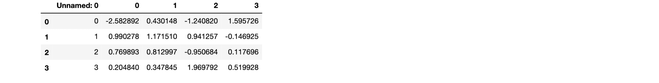
Yous tin can also salvage your array with the NumPy savetxt method.
>>> np . savetxt ( 'np.csv' , a , fmt = ' %.2f ' , delimiter = ',' , header = 'one, 2, iii, 4' ) If you're using the control line, you tin can read your saved CSV whatever fourth dimension with a command such as:
$ cat np.csv # 1, ii, iii, 4 -two.58,0.43,-1.24,1.60 0.99,ane.17,0.94,-0.15 0.77,0.81,-0.95,0.12 0.xx,0.35,i.97,0.52 Or y'all can open the file any fourth dimension with a text editor!
If you're interested in learning more than about Pandas, take a look at the official Pandas documentation. Learn how to install Pandas with the official Pandas installation information.
Plotting arrays with Matplotlib
If you need to generate a plot for your values, information technology's very simple with Matplotlib.
For example, y'all may take an array like this one:
>>> a = np . assortment ([ two , 1 , 5 , vii , four , 6 , 8 , 14 , 10 , ix , 18 , 20 , 22 ]) If you already have Matplotlib installed, you lot can import it with:
>>> import matplotlib.pyplot as plt # If you're using Jupyter Notebook, you may as well want to run the following # line of code to display your lawmaking in the notebook: %matplotlib inline All you demand to do to plot your values is run:
>>> plt . plot ( a ) # If you are running from a command line, you may demand to do this: # >>> plt.show() 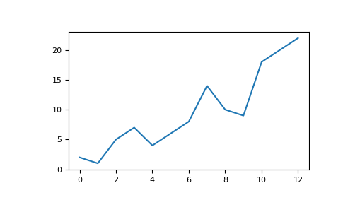
For example, you tin can plot a 1D array similar this:
>>> ten = np . linspace ( 0 , 5 , 20 ) >>> y = np . linspace ( 0 , ten , 20 ) >>> plt . plot ( x , y , 'purple' ) # line >>> plt . plot ( x , y , 'o' ) # dots 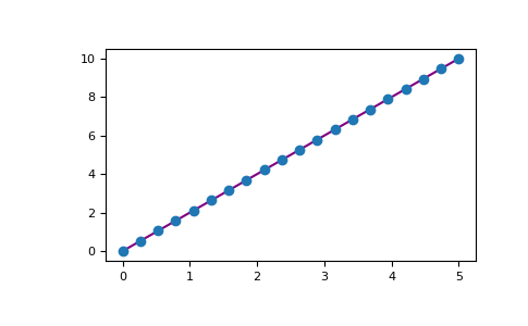
With Matplotlib, you have access to an enormous number of visualization options.
>>> fig = plt . figure () >>> ax = fig . add_subplot ( projection = '3d' ) >>> X = np . arange ( - 5 , five , 0.15 ) >>> Y = np . arange ( - 5 , 5 , 0.15 ) >>> X , Y = np . meshgrid ( 10 , Y ) >>> R = np . sqrt ( X ** two + Y ** 2 ) >>> Z = np . sin ( R ) >>> ax . plot_surface ( X , Y , Z , rstride = one , cstride = 1 , cmap = 'viridis' ) 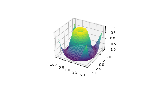
To read more than about Matplotlib and what it can do, take a look at the official documentation. For directions regarding installing Matplotlib, see the official installation section.
Image credits: Jay Alammar http://jalammar.github.io/
foresterbrounally43.blogspot.com
Source: https://numpy.org/devdocs/user/absolute_beginners.html
Posting Komentar untuk "How to Read 2d Data in Numpy"